Active Inference as a Convex Markov Decision Process
This paper discusses a new way to understand how agents can learn and make decisions by minimizing a measure called expected free energy. It connects this idea to existing methods in reinforcement learning, showing how they can work together.
Content & Liability Disclaimer
This article and its accompanying video are automated summaries derived from the original research paper by Unknown authors. The original research was conducted solely by the paper's authors; PDFdigest did not conduct any of the research and makes no claims of ownership over the underlying scientific work.
The video narration is generated by artificial intelligence and references the paper's authors for attribution. The video is not narrated by any of the paper's authors. This content may contain inaccuracies, omissions, or misinterpretations of the original research. First-person language (e.g., "we found", "our results") reflects the original authors' voice, not PDFdigest's. Always read the original paper for accurate, verified information before making any decisions based on this content.
This content is provided "as is" without any warranties, express or implied. Simulated systems OÜ, its officers, directors, employees, and agents shall not be liable for any direct, indirect, incidental, special, consequential, or punitive damages arising from your use of, reliance on, or access to this content, including but not limited to errors, omissions, or misinterpretations of the original research. This disclaimer applies to the fullest extent permitted by applicable law.
- 1 This can be read off immediately from the objective once the EFE is brought into its state-action marginal form.
- 2 The objective in standard MDPs is linear and the nonlinear case does not admit global value functions.
- 3 It is specialized by the EFE objective whose nonlinearity is the state-marginal negative entropy Φ.
- 4 Since entropy is not additive across the discount weights, the finitehorizon objective G = ⟨ℓ, µ⟩t H(ρ t ) has two inequivalent stationary analogues.
Methodology
We therefore leave a convergence analysis to future work. For each method at convergence (k = K), the per-step imagined state occupancy ρ t (s) is shown at five evenly spaced timesteps t ∈ {0, ⌊H/4⌋, ⌊H/2⌋, ⌊3H/4⌋, H} = {0, 3, 6, 9, 12}.
Study Design
We therefore leave a convergence analysis to future work.
Results & Findings
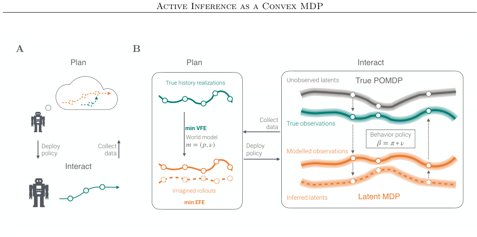
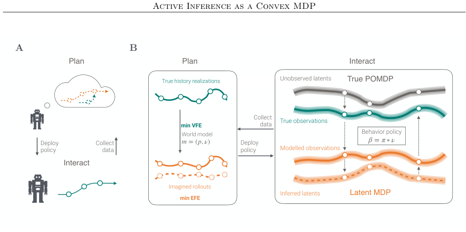
Model-based policy optimization (MBPO) lets an agent learn a world model from environment interaction and optimize a reactive policy on imagined rollouts inside that model. The two decision processes are coupled because the variational distribution ν is used in variational model learning and in action selection through the behavior policy β = π • ν.
- Model-based policy optimization (MBPO) lets an agent learn a world model from environment interaction and optimize a reactive policy on imagined rollouts inside that model.
- The two decision processes are coupled because the variational distribution ν is used in variational model learning and in action selection through the behavior policy β.
- The agent acts using the behavior policy β = π • ν, fits its model by Variational Free Energy (VFE) minimization to obtain m = (p.
- The agent learns a generative model of the environment and selects actions by minimising an expected free energy (EFE) that scores imagined future outcomes against a.
- Implementations use a recurrent world model, an actor, and a critic trained on imagined environment interactions.
We prove existence of a stable policy-model pair (Proposition 5) and leave convergence to future work.
Without action complexity, only the support-stationary point of (56), as (55) cannot populate an unplayed action.
Practical Applications
Generalizing to infinite horizons is possible but comes with modeling choices. The parameter-based novelty terms in the EFE may induce complex π-dependence.
How PDFdigest Helps You Understand Research
Instant Paper Analysis
Get structured summaries and key findings from dense PDFs in seconds.
Visual Explanations
Turn complex methods, figures, and results into clearer visual breakdowns.
AI-Powered Q&A
Ask focused questions and get answers grounded in the paper.
Contributions
The contributions section outlines the main findings: the structure of EFE as a convex functional, the development of a mirror-descent-inspired algorithm for EFE minimization, and the establishment of a performative policy-model pair under mild assumptions.
Episodic Active Inference
This section describes the episodic active inference framework, detailing the components of the POMDP and the behavior policy used by the agent. It explains the process of model learning and policy optimization in the context of active inference.
VFE: World Model Training
The VFE section explains the training of the world model through variational free energy minimization on real environment data. It discusses the generative model and recognition density used for inferring states.
Figures Explained
The paper’s visual material highlights the workflow and the main system components.
- Figure 1 :: Figure1: The episodic active inference setting considered in this work: A) the environment admits a true partially observable decision process, while the agent learns a latent fully observable process using variational inference. B) In contrast to standard variational inference, the two decision processes are coupled: the variational distribution ν is used both in variational model learning and in action selection through the behavior policy β = π • ν. The agent acts in the environment using the behavior policy β = π • ν for multiple episodes, then uses the data to fit its model by Variational Free Energy (VFE) minimization to obtain m = (p, ν), and uses that model to optimize its policy in imagination by minimizing the Expected Free Energy (EFE).
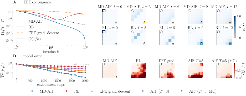
- 12 RLFigure 2 :: Figure 2: MD-AIF on gridworld environments. (A, top two rows) 5×5 deterministic gridworld. Left: EFE convergence (log-log scale) for MD-AIF, RL (no novelty), and EFE gradient descent, together with the theoretical O(1/k) rate (dashed). MD-AIF converges faster and to a lower value, driven by regularized dynamic programming. Right: Per-step imagined occupancy ρ t (s) at convergence (k = 100) for MD-AIF (top) and RL (bottom) at five timesteps t ∈ {0, 3, 6, 9, 12}. MD-AIF spreads probability mass broadly across the grid before concentrating toward the goal, whereas RL greedily channels mass along the direct path. Both rows share the same color scale. (B) 10 × 10 deterministic gridworld with uniform preference (pure epistemic drive). Left: Mean total-variation error TV(p, p ⋆ ) of the model fit as a function of environment steps under the interleaved model-policy loop. MD-AIF’s information-gain drive produces broader state coverage, accelerating model learning relative to RL and EFE gradient descent. AIF agents [2] plan myopically over short horizons (T = 3 exact; T = 5 via Monte Carlo with N mc = 100 samples). Right: Per-state model error TV(p, p ⋆ ) = E a∼π T TV(p(•|s, a), p ⋆ (•|s, a)) after 2500 environment steps.
- ) 5 🙂 6 :: π k+1 ← MD-AIF(π k ; m k+1 , pk+1 , T, η, q k+1 0 return π K To see this, consider the one pass of the full loop (2). Deploying π (behavior β = π•ν) in the real environment induces the history distribution D(π); the perception step returns the VFE-optimal model m ⋆ (D(π)) ∈ arg min m∈M F m; D(π) =: p π , ν π , and this refit model is what the planner sees: it supplies a linear pseudo-cost ℓ π and the augmented transition kernel P π of Lemma 6, ℓ π := ℓ m ⋆ (D(π)) , P π := p m ⋆ (D(π)) . Thus the decision-dependence is the composition π.
- Figure 4: s,a p(s ′ |s, a)π t (a|s)ρ t (s). Constant step size η = 0.05.Convergence plot. The y-axis shows Γ(ρ k ) -Γ ⋆ , where Γ ⋆ is the minimum across all three methods and all iterates. The O(1/k) reference line is fitted to MD-AIF’s initial gap: C/k with C = Γ(ρ 0 ) -Γ ⋆ . Both axes are logarithmic.
- 2 .: Deploy the resulting policy: sample E = 5 episodes of length H = 25 from the true environment by ancestral sampling (a t ∼ π t (•|s t ), s t+1 ∼ p ⋆ (•|s t , a t )).
Limitations and Cautions
A useful limitation and caution is that this article summarizes the available paper text and extracted evidence; readers should consult the source paper before treating any interpretation as definitive.
The paper’s conclusions may depend on its source selection, definitions, assumptions, and the scope of its analysis, so follow-up reading is important.
Source Paper Figures and Captions
![Figure 2: MD-AIF on gridworld environments. (A, top two rows) 5\\\\u00d75 deterministic gridworld. Left: EFE convergence (log-log scale) for MD-AIF, RL (no novelty), and EFE gradient descent, together with the theoretical O(1\\\\\\\/k) rate (dashed). MD-AIF converges faster and to a lower value, driven by regularized dynamic programming. Right: Per-step imagined occupancy \\\\u03c1 t (s) at convergence (k = 100) for MD-AIF (top) and RL (bottom) at five timesteps t \\\\u2208 {0, 3, 6, 9, 12}. MD-AIF spreads probability mass broadly across the grid before concentrating toward the goal, whereas RL greedily channels mass along the direct path. Both rows share the same color scale. (B) 10 \\\\u00d7 10 deterministic gridworld with uniform preference (pure epistemic drive). Left: Mean total-variation error TV(p, p \\\\u22c6 ) of the model fit as a function of environment steps under the interleaved model-policy loop. MD-AIF's information-gain drive produces broader state coverage, accelerating model learning relative to RL and EFE gradient descent. AIF agents [2] plan myopically over short horizons (T = 3 exact; T = 5 via Monte Carlo with N mc = 100 samples). Right: Per-state model error TV(p, p \\\\u22c6 ) = E a\\\\u223c\\\\u03c0 T TV(p(\\\\u2022|s, a), p \\\\u22c6 (\\\\u2022|s, a)) after 2500 environment steps.](https://pdfdigest.com/wp-content/uploads/nala/output/paper_dia5dL3xsSIMjvLZ_figure_02.png)
Frequently Asked Questions
This can be read off immediately from the objective once the EFE is brought into its state-action marginal form. The objective in standard MDPs is linear and the nonlinear case does not admit global value functions.
We therefore leave a convergence analysis to future work. For each method at convergence (k = K), the per-step imagined state occupancy ρ t (s) is shown at five evenly spaced timesteps t ∈ {0, ⌊H/4⌋, ⌊H/2⌋, ⌊3H/4⌋, H} = {0, 3.
However, the interesting question is whether the optimization problem remains well-posed if the agent is allowed to update its model during policy optimization, which would restore the AIF problem in full spirit. The log-preference is uniform (log p(s) = const) so the.
Generalizing to infinite horizons is possible but comes with modeling choices. MD-AIF is therefore an efficient implementation of Kakade’s natural policy gradient (NPG) on the EFE.
We prove existence of a stable policy-model pair (Proposition 5) and leave convergence to future work. Without action complexity, only the support-stationary point of (56), as (55) cannot populate an unplayed action.
This paper discusses a new way to understand how agents can learn and make decisions by minimizing a measure called expected free energy. It connects this idea to existing methods in reinforcement learning, showing how they can work together.